Introduction to Sampling-Based Motion Planning: The RRT Algorithm
The primary motivation for developing the RRT algorithm is to address kinodynamic systems in high-dimensional state spaces. These systems usually aim to generate open-loop trajectories that satisfy global obstacle constraints and local differential constraints, which are valuable in a wide variety of robotic applications. I won’t dive into too many details on the literature here, but if you are interested, I highly encourage you to read the original RRT papers [1][2]. There, you can find an extensive literature review and a solid background on how the authors’ ideas are built on a large foundation of related research.
The objective behind the algorithm is to naturally extendable to any general high-dimensional problems that may involve differential constraints. Compared to multi-query variants (i.e., multiple goal inputs or configurations) such as probabilistic roadmaps (PRMs), RRTs only aim to address single-query efficiently without any preprocessing requirments of the environment.
Notes on definitions and notations used
First, I’d like to start off the discussion by addressing the notation on state space. In robotics, especially in the motion planning community, the terms “configuration space” (also known as C-space) and “state space” are often used interchangeably, but they are not the same.
State space typically refers to the set of all possible states that a system can be in. For example, in the context of robotics, a state might include the positions and velocities of all the joints in a robotic arm. It’s essentially a representation of the complete snapshot of the system at a given moment.
On the other hand, the configuration space, also referred to as C-space, is a bit more specialized. It specifically refers to the set of all possible configurations that a system can have, without considering the details of how the system moves between configurations. In simpler terms, it’s a more abstract representation that focuses on the different possible arrangements of the system.
We use the notation $C$ to denote the configuration space (C-space). The expression $q \in C$ is commonly used to represent a configuration of a system within C-space. The symbol $X$ is used to represent the state space, in which a state, $x \in X$, can be expressed as $x = (q, \phantom{.}\smash{\dot{q}}, \phantom{.}\smash\ldots)$, i.e., it may include higher order derivatives as necessary, depending on the problem domain.
In order to simplify things here, I’m going to limit our problem domain into holonomic planning (i.e., there will be no differential constraints). Therefore, our planning state space can be expressed as in one variable $q$, i.e., $x = (q)$, where each $q \in C$ can be position and orientation of a geometric body of the robot in space.
Algorithm
The following pseudocode illustrates the basic concepts of the RRT algorithm.
RRT searches for a solution path to a planning problem by constructing a tree through a collision-free space from the start configuration state to the goal configuration state. This tree is incrementally built by randomly drawing samples from the problem domain.
We will use the notation $G$ to represent the tree, consisting of a set of vertices $V$ and edges $E$. First, the tree is initialized with a start configuration $x_{start}$ in the vertex set. In each iteration, the algorithm starts the tree construction process by randomly sampling a collision-free state $x_{rand}$ in the problem state space (Line 3). The randomly sampled state is then used to query the nearest neighbor vertex in the tree (Line 4). The function Steer in Line 5 generates a new state $x_{new}$ by making a motion toward $x_{rand}$ with a control input for some time increment. Here, we will assume the simple holonomic planning scenario with no differential constraints. Therefore, the potential new vertex $x_{new}$ can be simply connected from the nearest vertex $x_{nearest}$, limited by the distance $\Delta{d}$. The algorithm then performs collision checking of the edge $(x_{nearest}, x_{new})$ (Line 6). If this edge is collision-free, $x_{new}$ is added to the vertex set along with the edge, where $x_{new}$’s parent being $x_{nearest}$ (Lines 7-9). This vertex extension process of the RRT algorithm is illustrated in the following figure.
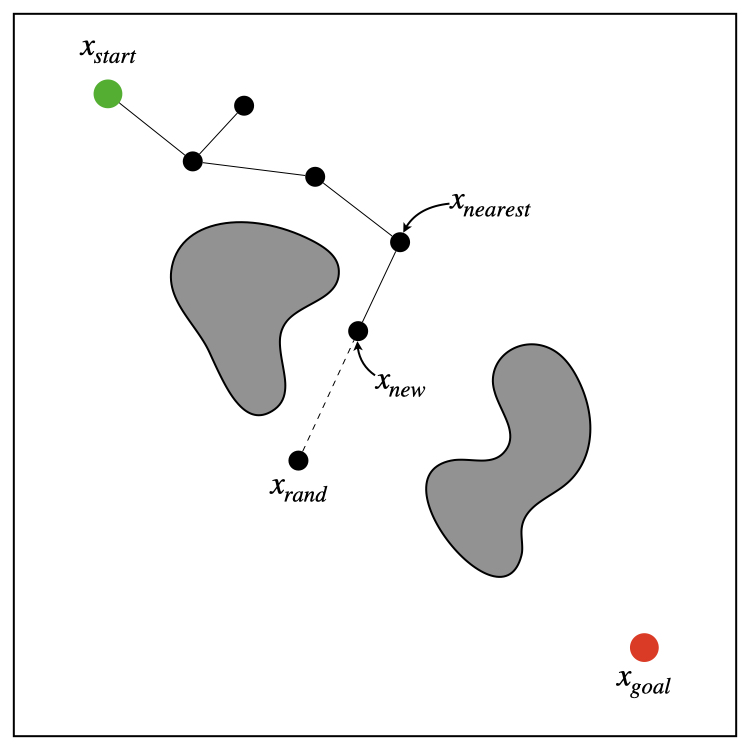 Vertex extension step of the RRT algorithm (aka EXTEND operation)
References
[1] LaValle, S. (1998). Rapidly-exploring random trees: A new tool for path planning. Research Report 9811.
[2] LaValle, S. M., & Kuffner Jr, J. J. (2001). Randomized kinodynamic planning. The international journal of robotics research, 20(5), 378-400.
[3] Kuffner, J. J., & LaValle, S. M. (2000, April). RRT-connect: An efficient approach to single-query path planning. In Proceedings 2000 ICRA. Millennium Conference. IEEE International Conference on Robotics and Automation. Symposia Proceedings (Cat. No. 00CH37065) (Vol. 2, pp. 995-1001). IEEE.