Notes on Multivariate Gaussians

Prerequisites

Linearity of Expectation

Linearity of expectation is the property that the expected value of the sum of random variables is equal to the sum of their individual expected values, regardless of whether they are independent.

For random variables $X$ and $Y$:

\[E[X + Y] = E[X] + E[Y]\]

In general, for any random variables $X_1, X_2, \dots, X_n$ and constants $c_1, c_2, \dots, c_n$:

\[E\left[ \sum_{i=1}^{n} c_i X_i \right] = \sum_{i=1}^{n} (c_i \cdot E[X_i]).\]

Random Vectors

A random vector $\mathbf{X}$ is a list of $n$ random variables defined in an $n \times 1$ (column) vector form:

\[\mathbf{X} = \left[ \begin{array}{c} X_1 \\ X_2 \\ \vdots \\ X_n \end{array} \right]\]

Expectation (mean)

The expectation (mean) of the random vector $\mathbf{X}$ is given by:

\[E[\mathbf{X}] = \left[ \begin{array}{c} E[X_1] \\ E[X_2] \\ \vdots \\ E[X_n] \end{array} \right]\]

The linearity properties of expectation can be applied to random vectors as well, for example:

\[E[A\mathbf{X}] = A \cdot E[\mathbf{X}]\] \[E[A\mathbf{X} + b] = A \cdot E[\mathbf{X}] + b\]

Covariance Matrix

The covariance matrix of the random vector $\mathbf{X}$ is given by:

\[Cov(\mathbf{X}) = E\left[ (\mathbf{X} - E[\mathbf{X}])(\mathbf{X} - E[\mathbf{X}])^\intercal \right]\]

It is an $n \times n$ symmetric matrix whose $(i, j)$ element is $Cov(X_i, X_j)$ and is a generalization of the variance of a random variable, i.e., $Var(X) = E[X^2] - (E[X])^2$. The $i^\text{th}$ diagonal element is the variance of $X_i$:

\[Cov(\mathbf{X}) = \left[ \begin{array}{c} Var(X_1) & Cov(X_1, X_2) & \cdots & Cov(X_1, X_n) \\ Cov(X_2, X_1) & Var(X_2) & \cdots & Cov(X_2, X_n) \\ \vdots & \vdots & \ddots & \vdots \\ Cov(X_n, X_1) & Cov(X_n, X_2) & \cdots & Var(X_n) \end{array} \right]\]

Affine Transformations

An affine transformation of the random vector involves a linear transformation followed by a translation.

Let $A$ be an $m \times n$ linear transformation matrix and $b$ be $m \times 1$ vector. If we apply this transformation to a random vector $\mathbf{X}$ and translated by a vector $b$, the $m \times 1$ affine transformed vector is given by $\mathbf{Y} = A \cdot \mathbf{X} + b$. Therefore, for the expectation (mean) of this transformed vector, we have:

\[E[\mathbf{Y}] = E[A \cdot \mathbf{X} + b]\]

If $\mathbf{Y}$ is a linear combination of $\mathbf{X}$, by linearity of expectation, we have:

\[E[\mathbf{Y}] = A \cdot E[\mathbf{X}] + b\]

For the covariance matrix, there is no effect of translation as it does not alter the dispersion or shape of the distribution. Therefore, we have:

\[\begin{aligned} Cov(\mathbf{Y}) = Cov(\mathbf{A \mathbf{X}}) &= E\left[ (A \mathbf{X} - E[A \mathbf{X}])(A \mathbf{X} - E[A \mathbf{X}])^\intercal \right] \\\ &= E\left[ (A \mathbf{X} - AE[\mathbf{X}])(A \mathbf{X} - AE[\mathbf{X}])^\intercal \right] \\\ &= E\left[ A(\mathbf{X} - E[\mathbf{X}])(\mathbf{X} - E[\mathbf{X}])^\intercal A^\intercal \right] \\\ &= A \, E\left[(\mathbf{X} - E[\mathbf{X}])(\mathbf{X} - E[\mathbf{X}])^\intercal \right] A^\intercal \\\ &= A \, Cov(\mathbf{X}) \, A^\intercal \end{aligned}\]

The Multivariate Normal Distribution

The random vector $\mathbf{X}$ has the multivariate normal (or Gaussian) distribution if the random variables $X_1$, $X_1$, $\dots$, $X_n$ are jointly normal or jointly Gaussian. Then, it has the following joint density function:

\[p(\mathbf{X} \mid \mu, \Sigma) = \frac{1}{(\sqrt{2 \pi})^{n}(\sqrt{\text{det}(\Sigma)})}\, \text{exp}\left(-\frac{1}{2}(\mathbf{X} - \mu)^\intercal {\Sigma}^{-1} (\mathbf{X} - \mu)\right)\]

where $\mu = E[\mathbf{X}]$ is an expectation (mean) vector of dimension $n$ and $\Sigma = Cov(\mathbf{X})$ is a $n \times n$ symmetric, positive semi-definite covariance matrix. We can also write this as $\mathbf{X} \sim \mathcal{N}(\mu, \Sigma)$.

It has the standard multivariate normal distribution if the random variables $X_1$, $X_1$, $\dots$, $X_n$ are independent identically distributed standard normal, i.e., $\mu = 0$ and $\Sigma = I_n$, the $n \times n$ identity matrix:

\[p(\mathbf{X} \mid \mu = 0, \Sigma = I_n) = \frac{1}{(\sqrt{2 \pi})^{n}}\, \text{exp}\left(-\frac{1}{2}(\mathbf{X})^\intercal (\mathbf{X})\right)\]

If $n$ becomes 1, this density formula above reduces to the univariate Gaussian distribution with mean $\mu$ and variance $\sigma^2$:

\[p(X \mid \mu, \sigma^2) = \frac{1}{\left(\sqrt{2 \pi \sigma^2}\right)}\, \text{exp}\left( -\frac{1}{2 \sigma^2}(X - \mu)^2 \right)\]

The graph of a Gaussian is a characteristic symmetric “bell curve” shape. Here, the argument of the expotential function $-\frac{1}{2 \sigma^2}(X - \mu)^2$ is a quadratic function of variable $X$. And since the coefficient of the quadratic term is negative, the parabola opens downwards:

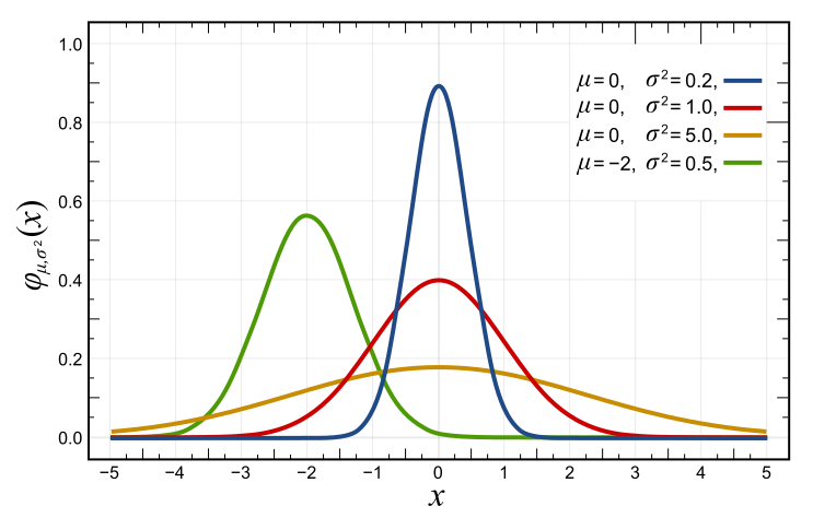Normalized Gaussian curves with expected value $\mu$ and variance $\sigma^2$ (Source: wikipedia).

The coefficient in front $\frac{1}{\left(\sqrt{2 \pi \sigma^2}\right)}$ is the normalizing constant which is used to ensure that the density function has the total probabilty of one, or in other words, its integral is 1:

\[\int_{-\infty}^{\infty} p(X \mid \mu, \sigma^2) = \frac{1}{\left(\sqrt{2 \pi \sigma^2}\right)}\, \int_{-\infty}^{\infty} \text{exp}\left( -\frac{1}{2 \sigma^2}(X - \mu)^2 \right) = 1\]

The same also applies to the multivariate Gaussian densities. The shape of the density is determined by the quadratic form $-\frac{1}{2}(\mathbf{X} - \mu)^\intercal {\Sigma}^{-1} (\mathbf{X} - \mu)$ and the level surfaces are ellipses and ellipsoids.

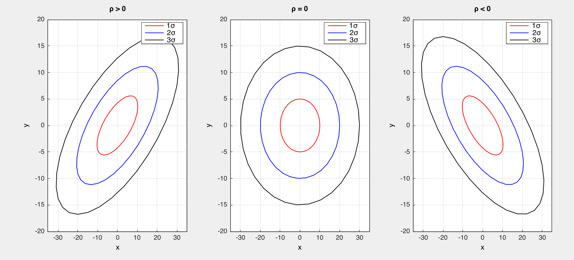2D Gaussians with different confidence levels (i.e. 68%, 90%, 95%) where the random variables are (1) positively correlated $\rho>0$, (2) independent $\rho=0$, and (3) negatively correlated $\rho<0$.