Understanding the Principle of Locality
Writing high-performance programs requires developers to understand a concept called locality, which enables programs to access data items that are in close proximity to recently accessed items. This notion, also widely known as the principle of locality, has a significant impact on designing performance-critical applications. In this article, I would like to briefly describe the fundamental idea of locality and provide some examples demonstrating how to write and evaluate locality-aware programs in C++.
Fundamental principles of locality
There are two main fundamental concepts in the principle of locality, namely temporal and spatial locality.
Temporal locality
Temporal locality refers to the tendency of a program to access the same memory locations repeatedly over a short period of time. In other words, if a program accesses a particular memory location, it is likely to access the same location again in the near future. This principle originates from the observation that programs often exhibit repetitive behavior, such as loops or frequently accessed variables. By exploiting temporal locality, programs can benefit from caching mechanisms that store recently accessed data in fast memory, reducing the time spent retrieving data from slower main memory or storage devices.
For example, consider a loop that iterates over an array to perform calculations. The loop repeatedly accesses elements of the array, exhibiting strong temporal locality. Caching mechanisms, such as CPU caches, take advantage of this repetitive access pattern by storing frequently accessed array elements in cache memory, thereby speeding up subsequent accesses and improving overall performance.
Spatial locality
Spatial locality refers to the tendency of a program to access data items that are stored close to each other in memory. When a program accesses a particular memory location, it is likely to access nearby memory locations in the near future. This principle originates from the observation that data elements in memory are often accessed sequentially or in close proximity due to the nature of program execution, such as iterating over arrays or traversing linked data structures.
For example, consider iterating over a two-dimensional array. As the program accesses elements of the array row by row, it exhibits strong spatial locality because nearby elements in memory are accessed sequentially. Spatial locality allows caching mechanisms to prefetch and cache contiguous blocks of memory, reducing the latency of memory accesses and improving overall efficiency.
Programmers should understand the principle of locality because, in general,
programs with good locality run faster than programs with poor locality.
Examples
Consider the following function that simply returns the sum of the elements of an input array of size N:
1
2
3
4
5
6
7
8
9
auto sumArray(const int arr[N])
{
    int sum = 0;

    for (size_t i = 0u; i < N; ++i)
        sum += arr[i];

    return sum;
}
Let’s evaluate this function to determine whether it has good locality by analyzing the access patterns of the variables. First, let’s examine the sum variable. This variable is repeatedly referenced inside each loop iteration, indicating that the function sumArray demonstrates good temporal locality with respect to sum. However, it does not have spatial locality since sum is a scalar variable.
In the case of the array variable arr, its elements are accessed sequentially, one after another, in each loop iteration. Therefore, we can infer that the function sumArray showcases good spatial locality with respect to arr, as each element in the array is stored contiguously in memory. However, it has poor temporal locality since each element of the array is accessed exactly once. Since the function sumArray demonstrates good temporal and/or spatial locality, we can conclude that this function has good locality.
Now, lets look at another example. Consider the following functions which sum up the two-dimensional array with two different access patterns:
1
2
3
4
5
6
7
8
9
10
11
12
13
14
15
16
17
18
19
20
21
auto sumArrayByRows(const int arr[M][N])
{
    int sum = 0;

    for (size_t i = 0u; i < M; ++i)
        for (size_t j = 0u; j < N; ++j)
            sum += arr[i][j];

    return sum;
}

auto sumArrayByCols(const int arr[M][N])
{
    int sum = 0;

    for (size_t j = 0u; j < N; ++j)
        for (size_t i = 0u; i < M; ++i)
            sum += arr[i][j];

    return sum;
}
Both functions correctly return the sum of the two-dimensional array; however they visit the elements of the array differently. The first function sumArrayByRows traverses the array in a row-major order, i.e., the inner loop iterates over each row first and then moves to the next row. On the other hand, the second function sumArrayByCols traverses the array in a column-major order, i.e., it iterates over each column first and then moves to the next column.
Since 2D arrays in C/C++ are allocated in row-major order (i.e., the memory layout consists of all the values in row 0 first, followed by the values in row 1, and so on), the first function sumArrayByRows enjoys good spatial locality as it accesses the array’s contents row by row. However, by simply changing the iteration pattern, as we can see in the second function sumArrayByCols, we encounter poor spatial locality because it accesses the contents column-wise instead of row-wise.
The following are the benchmark results for the two functions tested with 2D arrays of sizes 8, 32, 128, 512 and 1024. As we can see from the data, the function sumArrayByRows which does the row-major order traversal clearly outperforms the one with the column-major order traversal as the array size increases. Refer to Appendix section if you would like to replicate the results.
1
2
3
4
5
6
7
8
9
10
11
12
13
14
15
16
17
18
19
Run on (8 X 24 MHz CPU s)
CPU Caches:
  L1 Data 64 KiB
  L1 Instruction 128 KiB
  L2 Unified 4096 KiB (x8)
Load Average: 1.77, 2.08, 2.57
----------------------------------------------------------------------
Benchmark                            Time             CPU   Iterations
----------------------------------------------------------------------
BM_sumArrayByRows_8x8            0.404 ns        0.404 ns   1000000000
BM_sumArrayByRows_32x32           26.6 ns         26.6 ns     26290586
BM_sumArrayByRows_128x128         1321 ns         1321 ns       528031
BM_sumArrayByRows_512x512        12571 ns        12571 ns        55531
BM_sumArrayByRows_1024x1024      45409 ns        45409 ns        15409
BM_sumArrayByCols_8x8            0.404 ns        0.404 ns   1000000000
BM_sumArrayByCols_32x32            271 ns          271 ns      2586643
BM_sumArrayByCols_128x128         4192 ns         4192 ns       168758
BM_sumArrayByCols_512x512       150941 ns       150941 ns         4632
BM_sumArrayByCols_1024x1024     776507 ns       776507 ns          897
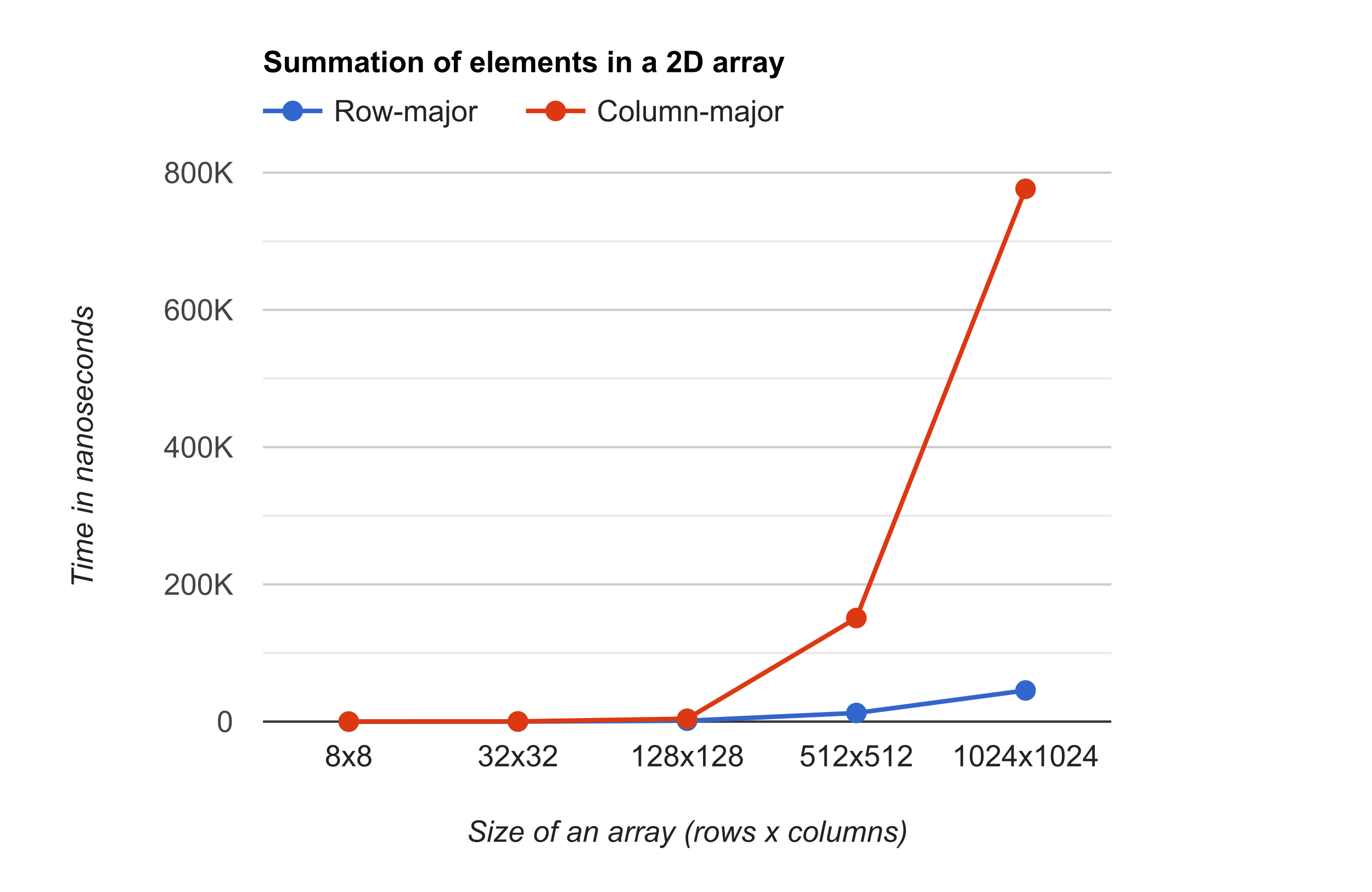 Performance comparsion results of row-major vs column-major in array traversal
Conclusion
So, how does it work? Why do programs with good temporal and spatial locality run faster? To answer these questions, we need to understand the underlying memory hierarchy that modern computing systems use to organize memory access and reduce the number of CPU clock cycles required to access data. In upcoming articles, we will look deeper into this memory hierarchy, also known as cache memories, and explore how to quantify the concept of locality in terms of cache hits and misses.
In any case, this article highlights the importance of quickly reviewing source code and having a general understanding of the program’s locality, which is a valuable and essential skill for programmers aiming to develop high-performance applications.
Appendix
If you would like to replicate the results, you can run the following script. Make sure to link against the Google Benchmark library during the build process. These benchmark results may vary from machine to machine. I ran those on my Macbook Air with a M2 chip using C++17 with Clang version 15.0.0 and optimization level -O3:
1
$ clang++ -std=c++17 -O3 -I <path-to-google-benchmark-include> -L <path-to-google-benchmark-lib> -lbenchmark sum_2darray_benchmark.cpp -o sum_2darray_benchmark